library(mice) #for imputation
library(summarytools) #for freq
library(dplyr) #other data management

dat <- rio::import("http://faculty.missouri.edu/huangf/data/kbbcarVALUE.xls")
summary(dat)
## Price Mileage Make Model
## Min. : 8639 Min. : 266 Length:804 Length:804
## 1st Qu.:14273 1st Qu.:14624 Class :character Class :character
## Median :18025 Median :20914 Mode :character Mode :character
## Mean :21343 Mean :19832
## 3rd Qu.:26717 3rd Qu.:25213
## Max. :70755 Max. :50387
## Trim Type Cylinder Liter
## Length:804 Length:804 Min. :4.000 Min. :1.600
## Class :character Class :character 1st Qu.:4.000 1st Qu.:2.200
## Mode :character Mode :character Median :6.000 Median :2.800
## Mean :5.269 Mean :3.037
## 3rd Qu.:6.000 3rd Qu.:3.800
## Max. :8.000 Max. :6.000
## Doors Cruise Sound Leather
## Min. :2.000 Min. :0.0000 Min. :0.0000 Min. :0.0000
## 1st Qu.:4.000 1st Qu.:1.0000 1st Qu.:0.0000 1st Qu.:0.0000
## Median :4.000 Median :1.0000 Median :1.0000 Median :1.0000
## Mean :3.527 Mean :0.7525 Mean :0.6791 Mean :0.7239
## 3rd Qu.:4.000 3rd Qu.:1.0000 3rd Qu.:1.0000 3rd Qu.:1.0000
## Max. :4.000 Max. :1.0000 Max. :1.0000 Max. :1.0000names(dat) <- tolower(names(dat))
dim(dat)## [1] 804 12freq(dat$cylinder)## Frequencies
## dat$cylinder
## Type: Numeric
##
## Freq % Valid % Valid Cum. % Total % Total Cum.
## ----------- ------ --------- -------------- --------- --------------
## 4 394 49.00 49.00 49.00 49.00
## 6 310 38.56 87.56 38.56 87.56
## 8 100 12.44 100.00 12.44 100.00
## <NA> 0 0.00 100.00
## Total 804 100.00 100.00 100.00 100.00freq(dat$leather)## Frequencies
## dat$leather
## Type: Numeric
##
## Freq % Valid % Valid Cum. % Total % Total Cum.
## ----------- ------ --------- -------------- --------- --------------
## 0 222 27.61 27.61 27.61 27.61
## 1 582 72.39 100.00 72.39 100.00
## <NA> 0 0.00 100.00
## Total 804 100.00 100.00 100.00 100.00dat$cylinder <- factor(dat$cylinder)comp.mod <- lm(price ~ mileage + leather + cylinder + cruise + liter, data = dat)Create some missing data
Create some missing data (randomly).
missing <- dat
set.seed(1234)
missing$cylinder[sample(nrow(dat), 100)] <- NA
missing$mileage[sample(nrow(dat), 50)] <- NA
missing$leather[sample(nrow(dat), 100)] <- NA
missing$liter[sample(nrow(dat), 100)] <- NA
miss.mod <- update(comp.mod, data = missing)

#export_summs(comp.mod, miss.mod) #this is in jtools
library(stargazer)
##
## Please cite as:## Hlavac, Marek (2018). stargazer: Well-Formatted Regression and Summary Statistics Tables.## R package version 5.2.2. https://CRAN.R-project.org/package=stargazerstargazer(comp.mod, miss.mod, no.space = T,
star.cutoffs = c(.05, .01, .001), type = 'text')##
## =====================================================================
## Dependent variable:
## -------------------------------------------------
## price
## (1) (2)
## ---------------------------------------------------------------------
## mileage -0.173*** -0.122***
## (0.028) (0.035)
## leather 906.268 681.713
## (543.292) (675.227)
## cylinder6 -711.765 -776.990
## (1,246.999) (1,626.238)
## cylinder8 15,834.910*** 17,676.030***
## (2,343.922) (3,031.968)
## cruise 6,864.731*** 6,666.896***
## (585.242) (732.340)
## liter 722.959 659.692
## (741.576) (969.586)
## Constant 15,068.880*** 14,438.220***
## (1,665.765) (2,151.273)
## ---------------------------------------------------------------------
## Observations 804 510
## R2 0.561 0.580
## Adjusted R2 0.557 0.575
## Residual Std. Error 6,576.985 (df = 797) 6,530.650 (df = 503)
## F Statistic 169.476*** (df = 6; 797) 115.755*** (df = 6; 503)
## =====================================================================
## Note: *p<0.05; **p<0.01; ***p<0.001Try to understand the pattern of missingness. How many complete cases do we have? 510 / 804 = 63%. Technically, (see other notes), the number of imputations will likely be m = (1 - %complete) * 100. For simplicity, we’ll just use 5 for now (it is easy to change).
md.pattern(missing, rotate.names = T) #rotate.names is in the updated version of mice
##     price make model trim type doors cruise sound mileage cylinder liter
## 510     1    1     1    1    1     1      1     1       1        1     1
## 65      1    1     1    1    1     1      1     1       1        1     1
## 64      1    1     1    1    1     1      1     1       1        1     0
## 17      1    1     1    1    1     1      1     1       1        1     0
## 73      1    1     1    1    1     1      1     1       1        0     1
## 11      1    1     1    1    1     1      1     1       1        0     1
## 12      1    1     1    1    1     1      1     1       1        0     0
## 2       1    1     1    1    1     1      1     1       1        0     0
## 39      1    1     1    1    1     1      1     1       0        1     1
## 4       1    1     1    1    1     1      1     1       0        1     1
## 4       1    1     1    1    1     1      1     1       0        1     0
## 1       1    1     1    1    1     1      1     1       0        1     0
## 2       1    1     1    1    1     1      1     1       0        0     1
##         0    0     0    0    0     0      0     0      50      100   100
##     leather
## 510       1   0
## 65        0   1
## 64        1   1
## 17        0   2
## 73        1   1
## 11        0   2
## 12        1   2
## 2         0   3
## 39        1   1
## 4         0   2
## 4         1   2
## 1         0   3
## 2         1   2
##         100 350
library(BaylorEdPsych)
lctest <- select(missing, mileage, leather, cylinder, cruise, liter, price) %>%
LittleMCAR() #test## this could take a whilelctest$chi.square## [1] 28.5983lctest$df## [1] 50lctest$p.value## [1] 0.9935462For the Little MCAR test, check the p value: it is not statisticaly significant, \(\chi^{2}(50) = 28.6, p = .99\), supporting the hypothesis that the data are missing completely at random: which it is since we deleted observations randomly.
NOTE: if data are MCAR– then just using listwise deletion (the default) is actually fine because results should not be biased. This may result though in lower power (since your complete case n is much lower).
We can however, also impute several datasets and analyze that. The following is the general workflow when using imputed data:
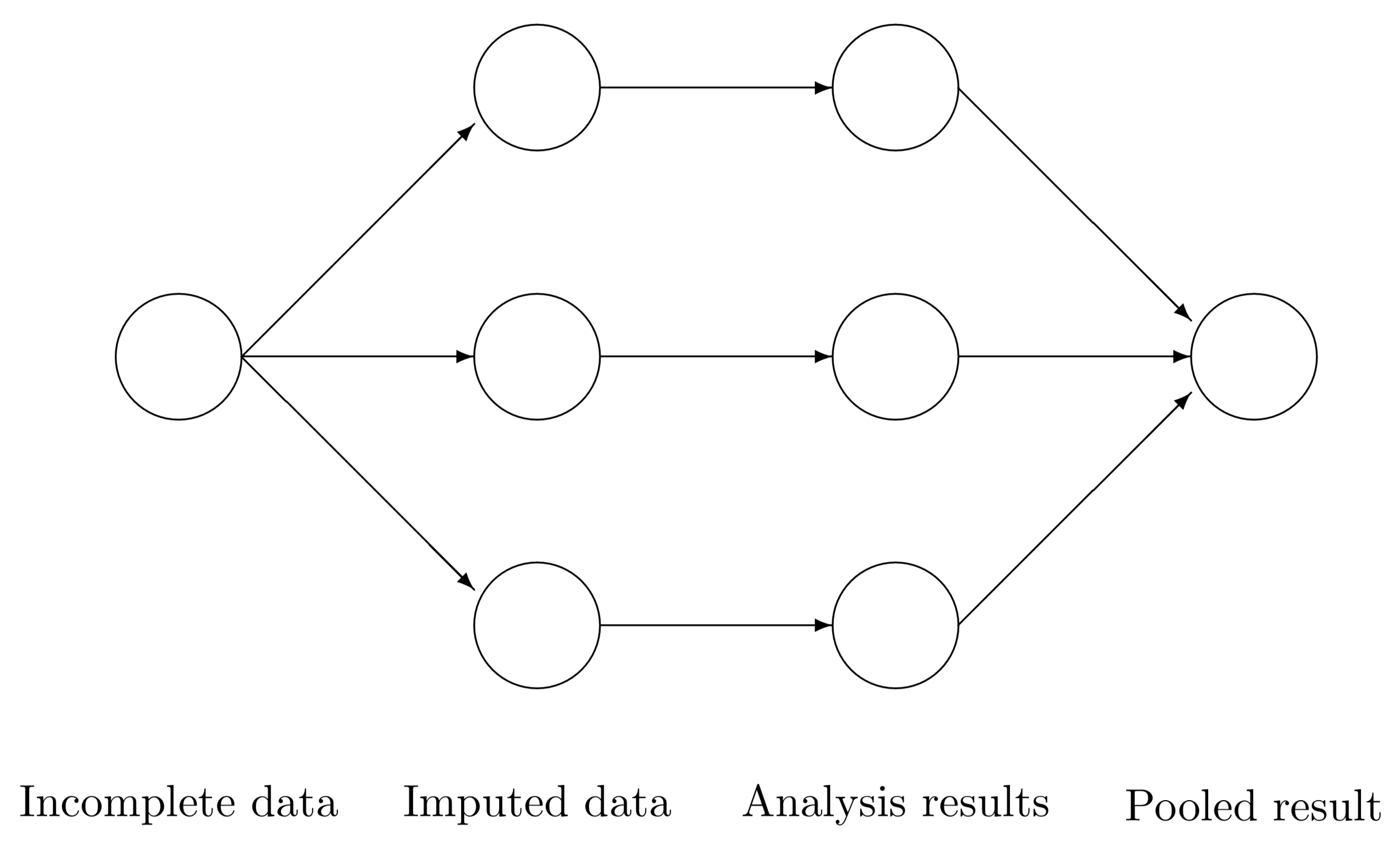
Impute missing data
Decide– how many datasets to impute and what kind of imputation to use. Understand what is missing and the missing data mechanism (see class notes).
imp <- mice(missing, m = 5) #5 imputations##
## iter imp variable
## 1 1 mileage cylinder liter leather
## 1 2 mileage cylinder liter leather
## 1 3 mileage cylinder liter leather
## 1 4 mileage cylinder liter leather
## 1 5 mileage cylinder liter leather
## 2 1 mileage cylinder liter leather
## 2 2 mileage cylinder liter leather
## 2 3 mileage cylinder liter leather
## 2 4 mileage cylinder liter leather
## 2 5 mileage cylinder liter leather
## 3 1 mileage cylinder liter leather
## 3 2 mileage cylinder liter leather
## 3 3 mileage cylinder liter leather
## 3 4 mileage cylinder liter leather
## 3 5 mileage cylinder liter leather
## 4 1 mileage cylinder liter leather
## 4 2 mileage cylinder liter leather
## 4 3 mileage cylinder liter leather
## 4 4 mileage cylinder liter leather
## 4 5 mileage cylinder liter leather
## 5 1 mileage cylinder liter leather
## 5 2 mileage cylinder liter leather
## 5 3 mileage cylinder liter leather
## 5 4 mileage cylinder liter leather
## 5 5 mileage cylinder liter leather## Warning: Number of logged events: 4### NOTE: it is very important that you set the variables to the proper type (factor vs numeric)
summary(imp)## Class: mids
## Number of multiple imputations: 5
## Imputation methods:
## price mileage make model trim type cylinder
## "" "pmm" "" "" "" "" "polyreg"
## liter doors cruise sound leather
## "pmm" "" "" "" "pmm"
## PredictorMatrix:
## price mileage make model trim type cylinder liter doors cruise
## price 0 1 0 0 0 0 1 1 1 1
## mileage 1 0 0 0 0 0 1 1 1 1
## make 1 1 0 0 0 0 1 1 1 1
## model 1 1 0 0 0 0 1 1 1 1
## trim 1 1 0 0 0 0 1 1 1 1
## type 1 1 0 0 0 0 1 1 1 1
## sound leather
## price 1 1
## mileage 1 1
## make 1 1
## model 1 1
## trim 1 1
## type 1 1
## Number of logged events: 4
## it im dep meth out
## 1 0 0 constant make
## 2 0 0 constant model
## 3 0 0 constant trim
## 4 0 0 constant typeViewing the summary shows that certain variables were imputed using pmm or predicted mean matching or some other method.
table(dat$cylinder)##
## 4 6 8
## 394 310 100table(dat$leather)##
## 0 1
## 222 582with(imp, table(cylinder)) #with is used to run the function with each multiply imputed dataset## call :
## with.mids(data = imp, expr = table(cylinder))
##
## call1 :
## mice(data = missing, m = 5)
##
## nmis :
## price mileage make model trim type cylinder liter
## 0 50 0 0 0 0 100 100
## doors cruise sound leather
## 0 0 0 100
##
## analyses :
## [[1]]
## cylinder
## 4 6 8
## 395 308 101
##
## [[2]]
## cylinder
## 4 6 8
## 389 313 102
##
## [[3]]
## cylinder
## 4 6 8
## 393 305 106
##
## [[4]]
## cylinder
## 4 6 8
## 391 311 102
##
## [[5]]
## cylinder
## 4 6 8
## 389 314 101with(imp, table(leather))## call :
## with.mids(data = imp, expr = table(leather))
##
## call1 :
## mice(data = missing, m = 5)
##
## nmis :
## price mileage make model trim type cylinder liter
## 0 50 0 0 0 0 100 100
## doors cruise sound leather
## 0 0 0 100
##
## analyses :
## [[1]]
## leather
## 0 1
## 218 586
##
## [[2]]
## leather
## 0 1
## 214 590
##
## [[3]]
## leather
## 0 1
## 226 578
##
## [[4]]
## leather
## 0 1
## 227 577
##
## [[5]]
## leather
## 0 1
## 231 573Leather is actually a factor so we should change that (if you don’t want to specify the imputation method manually).
missing$leather <- factor(missing$leather)Let’s try imputing again:
imp <- mice(missing, m = 5, seed = 123) #5 imputations, can set seed for reproducability##
## iter imp variable
## 1 1 mileage cylinder liter leather
## 1 2 mileage cylinder liter leather
## 1 3 mileage cylinder liter leather
## 1 4 mileage cylinder liter leather
## 1 5 mileage cylinder liter leather
## 2 1 mileage cylinder liter leather
## 2 2 mileage cylinder liter leather
## 2 3 mileage cylinder liter leather
## 2 4 mileage cylinder liter leather
## 2 5 mileage cylinder liter leather
## 3 1 mileage cylinder liter leather
## 3 2 mileage cylinder liter leather
## 3 3 mileage cylinder liter leather
## 3 4 mileage cylinder liter leather
## 3 5 mileage cylinder liter leather
## 4 1 mileage cylinder liter leather
## 4 2 mileage cylinder liter leather
## 4 3 mileage cylinder liter leather
## 4 4 mileage cylinder liter leather
## 4 5 mileage cylinder liter leather
## 5 1 mileage cylinder liter leather
## 5 2 mileage cylinder liter leather
## 5 3 mileage cylinder liter leather
## 5 4 mileage cylinder liter leather
## 5 5 mileage cylinder liter leather## Warning: Number of logged events: 4summary(imp)## Class: mids
## Number of multiple imputations: 5
## Imputation methods:
##     price   mileage      make     model      trim      type  cylinder
##        ""     "pmm"        ""        ""        ""        "" "polyreg"
##     liter     doors    cruise     sound   leather
##     "pmm"        ""        ""        ""  "logreg"
## PredictorMatrix:
## price mileage make model trim type cylinder liter doors cruise
## price 0 1 0 0 0 0 1 1 1 1
## mileage 1 0 0 0 0 0 1 1 1 1
## make 1 1 0 0 0 0 1 1 1 1
## model 1 1 0 0 0 0 1 1 1 1
## trim 1 1 0 0 0 0 1 1 1 1
## type 1 1 0 0 0 0 1 1 1 1
## sound leather
## price 1 1
## mileage 1 1
## make 1 1
## model 1 1
## trim 1 1
## type 1 1
## Number of logged events: 4
## it im dep meth out
## 1 0 0 constant make
## 2 0 0 constant model
## 3 0 0 constant trim
## 4 0 0 constant typeNOTE: in the way that the items are imputed, mice uses polytomous logistic regression and logistic regression– which is what we can expect when your data are multicategory or binary variables. THIS is important to know especially if you are imputing variables such as race or gender. Be cautious when imputing dummy coded variables if there are more than two categories (because this may not guarantee that you have one reference group).
with(imp, table(cylinder)) #with is used to run the function with each multiply imputed dataset## call :
## with.mids(data = imp, expr = table(cylinder))
##
## call1 :
## mice(data = missing, m = 5, seed = 123)
##
## nmis :
## price mileage make model trim type cylinder liter
## 0 50 0 0 0 0 100 100
## doors cruise sound leather
## 0 0 0 100
##
## analyses :
## [[1]]
## cylinder
## 4 6 8
## 391 312 101
##
## [[2]]
## cylinder
## 4 6 8
## 394 309 101
##
## [[3]]
## cylinder
## 4 6 8
## 392 310 102
##
## [[4]]
## cylinder
## 4 6 8
## 391 311 102
##
## [[5]]
## cylinder
## 4 6 8
## 394 307 103with(imp, table(leather))## call :
## with.mids(data = imp, expr = table(leather))
##
## call1 :
## mice(data = missing, m = 5, seed = 123)
##
## nmis :
## price mileage make model trim type cylinder liter
## 0 50 0 0 0 0 100 100
## doors cruise sound leather
## 0 0 0 100
##
## analyses :
## [[1]]
## leather
## 0 1
## 218 586
##
## [[2]]
## leather
## 0 1
## 232 572
##
## [[3]]
## leather
## 0 1
## 226 578
##
## [[4]]
## leather
## 0 1
## 221 583
##
## [[5]]
## leather
## 0 1
## 223 581with(imp, range(mileage))## call :
## with.mids(data = imp, expr = range(mileage))
##
## call1 :
## mice(data = missing, m = 5, seed = 123)
##
## nmis :
## price mileage make model trim type cylinder liter
## 0 50 0 0 0 0 100 100
## doors cruise sound leather
## 0 0 0 100
##
## analyses :
## [[1]]
## [1] 266 50387
##
## [[2]]
## [1] 266 50387
##
## [[3]]
## [1] 266 50387
##
## [[4]]
## [1] 266 50387
##
## [[5]]
## [1] 266 50387range(dat$mileage) #orig## [1] 266 50387densityplot(imp)
Selecting the imputation method manually
Users can also manually select the imputation method or variables to use for the prediction using the method and prediction matrices (see mice manual):
test <- mice(missing, m = 1)##
## iter imp variable
## 1 1 mileage cylinder liter leather
## 2 1 mileage cylinder liter leather
## 3 1 mileage cylinder liter leather
## 4 1 mileage cylinder liter leather
## 5 1 mileage cylinder liter leather## Warning: Number of logged events: 4(test$predictorMatrix) #can modify this## price mileage make model trim type cylinder liter doors cruise
## price 0 1 0 0 0 0 1 1 1 1
## mileage 1 0 0 0 0 0 1 1 1 1
## make 1 1 0 0 0 0 1 1 1 1
## model 1 1 0 0 0 0 1 1 1 1
## trim 1 1 0 0 0 0 1 1 1 1
## type 1 1 0 0 0 0 1 1 1 1
## cylinder 1 1 0 0 0 0 0 1 1 1
## liter 1 1 0 0 0 0 1 0 1 1
## doors 1 1 0 0 0 0 1 1 0 1
## cruise 1 1 0 0 0 0 1 1 1 0
## sound 1 1 0 0 0 0 1 1 1 1
## leather 1 1 0 0 0 0 1 1 1 1
## sound leather
## price 1 1
## mileage 1 1
## make 1 1
## model 1 1
## trim 1 1
## type 1 1
## cylinder 1 1
## liter 1 1
## doors 1 1
## cruise 1 1
## sound 0 1
## leather 1 0test$method## price mileage make model trim type cylinder
## "" "pmm" "" "" "" "" "polyreg"
## liter doors cruise sound leather
## "pmm" "" "" "" "logreg"Cylinder is actually an ordered, categorical variable. We can specify, let’s say, random forest imputation (note: the randomForest package has to be installed first.)
test$method["cylinder"] <- 'rf' #see ?mice
test$method
## price mileage make model trim type cylinder liter
## "" "pmm" "" "" "" "" "rf" "pmm"
## doors cruise sound leather
## "" "" "" "logreg"test2 <- mice(missing, method = test$method, printFlag = F)## Warning: Number of logged events: 4summary(test2)## Class: mids
## Number of multiple imputations: 5
## Imputation methods:
##    price  mileage     make    model     trim     type cylinder    liter
##       ""    "pmm"       ""       ""       ""       ""     "rf"    "pmm"
##    doors   cruise    sound  leather
##       ""       ""       "" "logreg"
## PredictorMatrix:
## price mileage make model trim type cylinder liter doors cruise
## price 0 1 0 0 0 0 1 1 1 1
## mileage 1 0 0 0 0 0 1 1 1 1
## make 1 1 0 0 0 0 1 1 1 1
## model 1 1 0 0 0 0 1 1 1 1
## trim 1 1 0 0 0 0 1 1 1 1
## type 1 1 0 0 0 0 1 1 1 1
## sound leather
## price 1 1
## mileage 1 1
## make 1 1
## model 1 1
## trim 1 1
## type 1 1
## Number of logged events: 4
## it im dep meth out
## 1 0 0 constant make
## 2 0 0 constant model
## 3 0 0 constant trim
## 4 0 0 constant typeAnalyze (imputed results)
Now, run a regression using the imputed datasets:
imp.mod <- with(imp, lm(price ~ mileage + leather + cylinder + cruise + liter)) #not data = statement since with is being used
#summary(imp.mod) #will show all regression results / dataset
What this is doing it running a regression m times (5 times), once with each imputed dataset. Results are then saved.
Pool results (using Rubin’s rules)
To report results– you have to pool the results using Rubin’s method (see far below) and then get the summary.
res <- pool(imp.mod) #no p values
round(summary(res), 3) #with p values, added the rounding so easier to read
## estimate std.error statistic df p.value
## (Intercept) 15019.508 1738.612 8.639 160.985 0.000
## mileage -0.177 0.029 -6.103 406.182 0.000
## leather1 1254.514 554.774 2.261 416.210 0.024
## cylinder6 -624.550 1323.521 -0.472 133.046 0.637
## cylinder8 15868.297 2489.954 6.373 125.336 0.000
## cruise 6885.198 584.604 11.778 772.834 0.000
## liter 653.135 780.852 0.836 145.733 0.403pool.r.squared(imp.mod) ## est lo 95 hi 95 fmi
## R^2 0.5671685 0.5196223 0.6116927 NaN#compare
#export_summs(comp.mod, miss.mod, model.names = c('complete', ' missing')) #this is in jtools-- usually do this but produces funny results when I knit the document
#cannot add pooled info side by side now
stargazer(comp.mod, miss.mod, star.cutoffs = c(.05, .01, .001), no.space = T, type = 'text')##
## =====================================================================
## Dependent variable:
## -------------------------------------------------
## price
## (1) (2)
## ---------------------------------------------------------------------
## mileage -0.173*** -0.122***
## (0.028) (0.035)
## leather 906.268 681.713
## (543.292) (675.227)
## cylinder6 -711.765 -776.990
## (1,246.999) (1,626.238)
## cylinder8 15,834.910*** 17,676.030***
## (2,343.922) (3,031.968)
## cruise 6,864.731*** 6,666.896***
## (585.242) (732.340)
## liter 722.959 659.692
## (741.576) (969.586)
## Constant 15,068.880*** 14,438.220***
## (1,665.765) (2,151.273)
## ---------------------------------------------------------------------
## Observations 804 510
## R2 0.561 0.580
## Adjusted R2 0.557 0.575
## Residual Std. Error 6,576.985 (df = 797) 6,530.650 (df = 503)
## F Statistic 169.476*** (df = 6; 797) 115.755*** (df = 6; 503)
## =====================================================================
## Note: *p<0.05; **p<0.01; ***p<0.001Creating nicer output
The section below just illustrates the findings using texreg for laying out the results (w/c are the same as what is shown above).
library(texreg)## Version: 1.36.23
## Date: 2017-03-03
## Author: Philip Leifeld (University of Glasgow)
##
## Please cite the JSS article in your publications -- see citation("texreg").tmp <- summary(res)
tr <- createTexreg(coef.names = row.names(tmp), coef = tmp[,1], se = tmp[,2],
pvalues = tmp[,5], gof.names = 'R2', gof = pool.r.squared(imp.mod)[1])
screenreg(tr, digits = 3)##
## ==========================
## Model 1
## --------------------------
## (Intercept) 15019.508 ***
## (1738.612)
## mileage -0.177 ***
## (0.029)
## leather1 1254.514 *
## (554.774)
## cylinder6 -624.550
## (1323.521)
## cylinder8 15868.297 ***
## (2489.954)
## cruise 6885.198 ***
## (584.604)
## liter 653.135
## (780.852)
## --------------------------
## R2 0.567
## ==========================
## *** p < 0.001, ** p < 0.01, * p < 0.05Results are combined with what is known as Rubin’s rules. Getting the regression coefficients is simple: just average all the values. Take for example the imputed results for liter B = 653, SE = 781.
res2 <- summary(imp.mod) #save all coefficients
### look at the res object to understand what is going on
res has all the coefficients for each model run. Let’s just focus on the liter variable.
Example
filter(res2, term == 'liter')## # A tibble: 5 x 5
## term estimate std.error statistic p.value
## <chr> <dbl> <dbl> <dbl> <dbl>
## 1 liter 559. 716. 0.781 0.435
## 2 liter 716. 738. 0.971 0.332
## 3 liter 353. 718. 0.492 0.623
## 4 liter 553. 722. 0.767 0.444
## 5 liter 1084. 712. 1.52 0.129There is some variability for liter!
filter(res2, term == 'liter') %>%
  summarise(m.est = mean(estimate),
            m.se = mean(std.error)) #this is the wrong SE, just showing
## # A tibble: 1 x 2
## m.est m.se
## <dbl> <dbl>
## 1 653. 721.The m.est is the same–> referred to as \((\bar{Q})\) where each \(Q\) is a coefficient. The standard error is not correct (721 vs 781). To compute the correct standard error, need to get the square root of the total variance associated with coefficient:
\(T = \bar{U} + (1 + \frac{1}{m})B\)
where \(T\) is the total variance. \(B\) is merely the variance of the regression coefficients (the coefficients are referred to as \(Q\)). \(\bar{U}\) is the mean of the variance of each cofficient (or the average of the square of the standard errors of each coefficient). To see this manually:
tmp <- filter(res2, term == 'liter') %>%
  select(estimate, std.error) #create a dataset with only the coefficients and standard errors for liter
(Bs <- var(tmp$estimate)) #variance of the coefficients
## [1] 74590.63The weighting by the number of imputations is specified by Rubin’s rules where \(m\) = number of imputations: \((1 + \frac{1}{m})\). In our case, m = 5.
(Ubar <- mean(tmp$std.error^2))## [1] 520221.3(se.imp <- (Ubar + (1 + 1/5) * Bs) %>% sqrt()) #compare this to the standard error of the imputed datasets## [1] 780.8521The t statistic is simply \(t(df) = \frac{\bar{Q}}{\sqrt{T}}\).
Others: Extracting datasets
Viewing the complete dataset:
To extract the imputed datasets, use the complete function. If you indicate action = 0, the original dataset will get extracted. If action = 1 then the first imputed dataset gets extracted, etc.. Using action = 'long' extracts all the datasets. You can still use the extracted datasets and then put them back as a mids object using the as.mids function.
alldat <- complete(imp, action = 'long')
freq(alldat$.imp)
## Frequencies
## alldat$.imp
##
## Freq % Valid % Valid Cum. % Total % Total Cum.
## ----------- ------ --------- -------------- --------- --------------
## 1 804 20.00 20.00 20.00 20.00
## 2 804 20.00 40.00 20.00 40.00
## 3 804 20.00 60.00 20.00 60.00
## 4 804 20.00 80.00 20.00 80.00
## 5 804 20.00 100.00 20.00 100.00
## <NA> 0 0.00 100.00
## Total 4020 100.00 100.00 100.00 100.00#str(alldat)
head(alldat) #has a .imp variable which says which imputation was used## .imp .id price mileage make model trim type cylinder liter
## 1 1 1 17314.10 8221 Buick Century Sedan 4D Sedan 6 3.1
## 2 1 2 17542.04 9135 Buick Century Sedan 4D Sedan 6 3.1
## 3 1 3 16218.85 13196 Buick Century Sedan 4D Sedan 6 3.8
## 4 1 4 16336.91 16342 Buick Century Sedan 4D Sedan 6 3.1
## 5 1 5 16339.17 19832 Buick Century Sedan 4D Sedan 6 3.1
## 6 1 6 15709.05 22236 Buick Century Sedan 4D Sedan 6 3.1
## doors cruise sound leather
## 1 4 1 1 1
## 2 4 1 1 0
## 3 4 1 1 0
## 4 4 1 0 0
## 5 4 1 0 1
## 6 4 1 1 0tail(alldat)## .imp .id price mileage make model trim type
## 4015 5 799 16425.17 14242 Saturn L Series L300 Sedan 4D Sedan
## 4016 5 800 16507.07 16229 Saturn L Series L300 Sedan 4D Sedan
## 4017 5 801 16175.96 19095 Saturn L Series L300 Sedan 4D Sedan
## 4018 5 802 15731.13 20484 Saturn L Series L300 Sedan 4D Sedan
## 4019 5 803 15118.89 25979 Saturn L Series L300 Sedan 4D Sedan
## 4020 5 804 13585.64 35662 Saturn L Series L300 Sedan 4D Sedan
## cylinder liter doors cruise sound leather
## 4015 6 3 4 1 0 0
## 4016 6 3 4 1 0 0
## 4017 6 3 4 1 1 0
## 4018 6 3 4 1 1 0
## 4019 6 3 4 1 1 0
## 4020 6 3 4 1 0 0This is useful if you want to do some post-processing of your data after imputation. There is much more to learn about missing data!
densityplot(imp, ~mileage) #viewing the imputed variables vs the original
Using Full Information Maximum Likelihood
This is also popular (especially among Mplus users) since you don’t have to do the impute, pool, and analyze steps (w/c sounds so much simpler!). Can also do this using lavaan. There are some things to watch out for though. I don’t generally use this in R.
library(lavaan)## This is lavaan 0.6-4## lavaan is BETA software! Please report any bugs.### NOTE: if you do it this way, you have to convert factors into dummy codes
fiml.dat <- dat
table(fiml.dat$cylinder)##
## 4 6 8
## 394 310 100fiml.dat$cyl6 <- ifelse(fiml.dat$cylinder == 6, 1, 0)
fiml.dat$cyl8 <- ifelse(fiml.dat$cylinder == 8, 1, 0)
table(fiml.dat$cyl6)##
## 0 1
## 494 310table(fiml.dat$cyl8)##
## 0 1
## 704 100### have to convert the price and mileage into something smaller,
### somehow, lavaan complains if the variance between variables is
### to different
fiml.dat$pr <- fiml.dat$price / 1000
fiml.dat$mi <- fiml.dat$mileage / 1000
mod1 <- '
pr ~ mi + leather + cyl6 + cyl8 + cruise + liter
'
res1 <- sem(model = mod1, data = fiml.dat)
summary(res1)## lavaan 0.6-4 ended normally after 54 iterations
##
## Optimization method NLMINB
## Number of free parameters 7
##
## Number of observations 804
##
## Estimator ML
## Model Fit Test Statistic 0.000
## Degrees of freedom 0
##
## Parameter Estimates:
##
## Information Expected
## Information saturated (h1) model Structured
## Standard Errors Standard
##
## Regressions:
## Estimate Std.Err z-value P(>|z|)
## pr ~
## mi -0.173 0.028 -6.139 0.000
## leather 0.906 0.541 1.675 0.094
## cyl6 -0.712 1.242 -0.573 0.566
## cyl8 15.835 2.334 6.785 0.000
## cruise 6.865 0.583 11.781 0.000
## liter 0.723 0.738 0.979 0.327
##
## Variances:
## Estimate Std.Err z-value P(>|z|)
## .pr 42.880 2.139 20.050 0.000Create missing values:
small <- select(fiml.dat, pr, mi, leather, cyl6, cyl8, cruise, liter)
set.seed(246)
small$cyl6[sample(nrow(small), 50)] <- NA #doing this separately for cylinder
small$cyl8[sample(nrow(small), 50)] <- NA
small$mi[sample(nrow(small), 50)] <- NA
small$leather[sample(nrow(small), 100)] <- NA
small$liter[sample(nrow(small), 100)] <- NA
md.pattern(small, rotate.names = T)
##     pr cruise mi cyl6 cyl8 leather liter
## 505  1      1  1    1    1       1     1   0
## 74   1      1  1    1    1       1     0   1
## 69   1      1  1    1    1       0     1   1
## 13   1      1  1    1    1       0     0   2
## 35   1      1  1    1    0       1     1   1
## 3    1      1  1    1    0       1     0   2
## 7    1      1  1    1    0       0     1   2
## 34   1      1  1    0    1       1     1   1
## 5    1      1  1    0    1       1     0   2
## 6    1      1  1    0    1       0     1   2
## 1    1      1  1    0    0       1     1   2
## 2    1      1  1    0    0       0     1   3
## 40   1      1  0    1    1       1     1   1
## 4    1      1  0    1    1       1     0   2
## 2    1      1  0    1    1       0     1   2
## 1    1      1  0    1    0       1     1   2
## 1    1      1  0    1    0       1     0   3
## 1    1      1  0    0    1       1     1   2
## 1    1      1  0    0    1       0     1   3
##      0      0 50   50   50     100   100 350
Using lavaan again:
mod2 <- '
pr ~ mi + leather + cyl6 + cyl8 + cruise + liter
'
res2 <- sem(model = mod2, data = small)
summary(res2)
## lavaan 0.6-4 ended normally after 55 iterations
##
## Optimization method NLMINB
## Number of free parameters 7
##
## Used Total
## Number of observations 505 804
##
## Estimator ML
## Model Fit Test Statistic 0.000
## Degrees of freedom 0
##
## Parameter Estimates:
##
## Information Expected
## Information saturated (h1) model Structured
## Standard Errors Standard
##
## Regressions:
## Estimate Std.Err z-value P(>|z|)
## pr ~
## mi -0.159 0.034 -4.600 0.000
## leather 0.961 0.673 1.427 0.154
## cyl6 0.107 1.547 0.069 0.945
## cyl8 19.279 2.925 6.591 0.000
## cruise 7.156 0.728 9.829 0.000
## liter -0.193 0.924 -0.209 0.834
##
## Variances:
## Estimate Std.Err z-value P(>|z|)
## .pr 42.481 2.673 15.890 0.000How to “turn on” FIML?
Specify, missing = 'fiml' and fixed.x = F (adds the covariances between variables in the output)
mod2 <- '
pr ~ mi + leather + cyl6 + cyl8 + cruise + liter
'
res3 <- sem(model = mod2, data = small, missing = 'fiml', fixed.x = F)
summary(res3)
## lavaan 0.6-4 ended normally after 114 iterations
##
## Optimization method NLMINB
## Number of free parameters 35
##
## Number of observations 804
## Number of missing patterns 19
##
## Estimator ML
## Model Fit Test Statistic 0.000
## Degrees of freedom 0
##
## Parameter Estimates:
##
## Information Observed
## Observed information based on Hessian
## Standard Errors Standard
##
## Regressions:
## Estimate Std.Err z-value P(>|z|)
## pr ~
## mi -0.179 0.029 -6.178 0.000
## leather 0.958 0.573 1.673 0.094
## cyl6 0.060 1.361 0.044 0.965
## cyl8 17.568 2.603 6.749 0.000
## cruise 6.965 0.584 11.917 0.000
## liter 0.159 0.820 0.194 0.846
##
## Covariances:
## Estimate Std.Err z-value P(>|z|)
## mi ~~
## leather -0.029 0.142 -0.204 0.838
## cyl6 -0.136 0.146 -0.928 0.354
## cyl8 -0.066 0.097 -0.681 0.496
## cruise 0.106 0.128 0.829 0.407
## liter -0.289 0.331 -0.874 0.382
## leather ~~
## cyl6 -0.043 0.008 -5.046 0.000
## cyl8 0.036 0.006 6.226 0.000
## cruise -0.011 0.007 -1.514 0.130
## liter 0.049 0.019 2.565 0.010
## cyl6 ~~
## cyl8 -0.048 0.006 -8.011 0.000
## cruise 0.045 0.008 5.933 0.000
## liter 0.220 0.021 10.609 0.000
## cyl8 ~~
## cruise 0.031 0.005 5.968 0.000
## liter 0.255 0.016 16.194 0.000
## cruise ~~
## liter 0.181 0.018 9.986 0.000
##
## Intercepts:
## Estimate Std.Err z-value P(>|z|)
## .pr 16.297 1.813 8.991 0.000
## mi 19.863 0.298 66.658 0.000
## leather 0.716 0.017 42.253 0.000
## cyl6 0.386 0.017 22.276 0.000
## cyl8 0.124 0.012 10.668 0.000
## cruise 0.752 0.015 49.440 0.000
## liter 3.037 0.039 77.371 0.000
##
## Variances:
## Estimate Std.Err z-value P(>|z|)
## .pr 42.479 2.137 19.874 0.000
## mi 67.159 3.459 19.415 0.000
## leather 0.204 0.011 18.749 0.000
## cyl6 0.238 0.012 19.779 0.000
## cyl8 0.108 0.005 19.876 0.000
## cruise 0.186 0.009 20.050 0.000
## liter 1.219 0.062 19.770 0.000Can also use auxilliary variables (in the semTools package). sem.auxilliary.